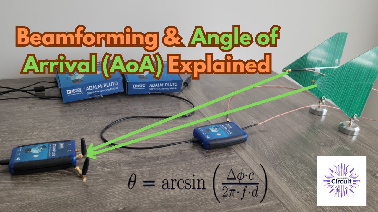
Traditional antennas are not especially picky. They transmit energy in broad patterns and listen to signals arriving from many directions, rather like someone shouting into a crowded restaurant and hoping the correct person hears the order. Beamforming changes that behavior. By coordinating multiple antenna elements, a radio can emphasize signals in a chosen direction, suppress interference elsewhere, and electronically steer its coverage without rotating a dish or asking an intern to move the antenna three degrees to the left.

Software-defined radio, or SDR, makes this capability far more flexible. Instead of locking modulation, filtering, synchronization, and array processing into fixed hardware, an SDR moves much of the signal chain into programmable processors. Engineers can test a basic delay-and-sum beamformer in the morning, experiment with adaptive null steering after lunch, and accidentally spend the evening debugging a clock cable that was loose the entire time.

Real-time beamforming with software-defined radio is now central to wireless research, phased-array radar, satellite communications, direction finding, spectrum monitoring, massive MIMO, and emerging sensing-and-communications systems. The exciting part is not merely forming a directional beam. The real challenge is estimating where the beam should point, calculating new coefficients, applying them across synchronized radio channels, and doing all of it before the propagation environment changes.

What Real-Time Beamforming Actually Does

Beamforming is a spatial filtering technique. An array receives slightly different versions of the same wave at each antenna because the wavefront reaches the elements at different times. By applying a carefully selected delay, phase shift, and amplitude weight to every channel, the receiver can align signals arriving from one direction. Those aligned signals combine constructively, while signals from other directions tend to combine less effectively or cancel.

The same principle works in transmission. Each antenna emits a version of the waveform with a controlled phase or delay. In the desired direction, the separate wavefronts arrive in step and reinforce one another. Elsewhere, they are misaligned. The result is an electronically steerable radiation pattern containing a main lobe, sidelobes, and, when deliberately designed, deep nulls toward interferers. Analog Devices describes this combination of channel gain and phase adjustment as the foundation of real-time electronic beam steering.

A Simple Four-Element Example

Consider a four-element uniform linear array operating at 2.45 GHz. The wavelength is approximately 12.24 centimeters, so half-wavelength element spacing is about 6.12 centimeters. To steer a narrowband beam approximately 30 degrees away from broadside, the array requires a progressive phase change of roughly 90 degrees between adjacent elements. The positive or negative sign depends on the transmit-versus-receive convention and the coordinate system.

The beamformer therefore applies a sequence resembling 0, 90, 180, and 270 degrees across the array. Change that progression in software and the beam moves. No gears, belts, bearings, or dramatic mechanical groaning are required.

Why Software-Defined Radio Is a Natural Beamforming Platform

An SDR generally combines an RF front end, data converters, programmable digital processing, and a software-accessible control interface. The radio tunes, amplifies, digitizes, and transports complex in-phase and quadrature samples. Software or programmable logic then performs channelization, filtering, demodulation, synchronization, array processing, and application-specific analysis.

Platforms in the USRP family, for example, use a common hardware-driver environment that supports frameworks such as GNU Radio, C++, Python, MATLAB, and other development tools. Modern devices may also include large FPGAs or RF system-on-chip processors, allowing critical DSP functions to run close to the converters instead of traveling through a host computer first.

This programmability gives SDR beamforming several advantages:

• Beam directions can be changed dynamically through software commands.
• Researchers can switch between conventional and adaptive algorithms.
• Multiple simultaneous receive beams can be created in the digital domain.
• Calibration coefficients can be updated as temperature and hardware behavior change.
• The same radio platform can support communications, radar, sensing, and direction-finding experiments.

The word “software” does not mean the antennas have become optional. It means the radio’s behavior can be reconfigured without redesigning every circuit. The RF chain still matters enormously, and it has many opportunities to remind the programmer that physics does not accept software patches.

Analog, Digital, and Hybrid Beamforming

Analog Beamforming

In an analog array, phase shifters and gain-control devices manipulate RF or intermediate-frequency signals before the antenna channels are combined. Because the receiver may need only one data-converter path for an entire subarray, analog beamforming can reduce cost, digital bandwidth, power consumption, and processing requirements.

The compromise is flexibility. A single analog network commonly forms one beam at a time, and the precision is limited by phase-shifter resolution, gain accuracy, component tolerances, and RF bandwidth. Analog beamforming remains attractive for large millimeter-wave arrays, where providing a complete high-speed digital chain for every element can become expensive and power hungry.

Digital Beamforming

Digital beamforming preserves a separate digitized channel for each antenna element or subarray. Complex weights are applied numerically, allowing the system to form several beams, adaptively suppress interference, and use different coefficients across frequency bins.

The price is data volume. Eight channels sampled at 100 million complex samples per second with 16-bit I and 16-bit Q values produce a raw rate of 25.6 gigabits per second before protocol overhead. Sending that fire hose through a modest USB connection is a splendid way to discover dropped samples.

Hybrid Beamforming

Hybrid beamforming divides the work between analog and digital stages. Groups of elements are combined through analog phase control, while a smaller number of digital RF chains perform precoding, combining, multiuser processing, or adaptive correction. This architecture is especially useful when arrays contain dozens or hundreds of elements but the system cannot afford an independent converter and full-rate processor for every antenna.

Practical millimeter-wave prototypes have combined software-controlled phased arrays with USRP hardware to evaluate beam training, channel estimation, and directional communication at 60 GHz. Such systems demonstrate why hybrid architecture is not merely a compromise; it is often the practical bridge between a beautiful simulation and hardware that can operate without requiring its own power station.

The Real-Time Signal-Processing Pipeline

A functional SDR beamformer is more than a block labeled “apply weights.” It is a continuous processing loop with strict timing requirements.

1. Acquire Coherent Array Samples

Every receiver channel must sample the same event using a common and stable time reference. The channels also need predictable phase relationships. Depending on the platform, this may require a shared reference clock, synchronized sample clocks, aligned local oscillators, deterministic start commands, timestamped streaming, or dedicated synchronization hardware.

Frequency synchronization alone is insufficient. Two receivers can be tuned to the same nominal carrier and still begin with unrelated phase offsets. If those offsets change after every restart, yesterday’s calibration values become decorative rather than useful.

2. Calibrate Gain, Phase, and Delay

Real RF channels are not identical. Cables have different electrical lengths. Mixers, filters, amplifiers, connectors, and converters introduce channel-dependent gain and phase responses. These errors can also drift with frequency, temperature, and time.

Calibration typically injects or receives a known reference signal, measures each channel relative to a selected reference path, and stores complex correction coefficients. Wideband systems may require frequency-dependent calibration rather than one coefficient per channel. Analog Devices notes that phased-array channel responses contain practical mismatches and time-varying errors that must be measured and corrected.

3. Estimate Direction or Channel State

A fixed beamformer may already know its desired steering direction. An adaptive system must estimate it. Common approaches include conventional beam scanning, monopulse processing, MUSIC, ESPRIT, channel sounding, pilot-based estimation, and codebook search.

MUSIC can provide high-resolution direction-of-arrival estimates by separating estimated signal and noise subspaces. However, it requires a reliable covariance matrix and additional matrix computation. MathWorks demonstrates practical MUSIC-based direction estimation using phase-coherent USRP receiver channels, illustrating the connection between array theory and deployable SDR measurements.

4. Calculate Beamforming Weights

The simplest method is conventional delay-and-sum beamforming. Steering-vector coefficients align the desired signal, and the weighted channels are added. This approach is inexpensive, predictable, and often the best place to begin.

Adaptive methods use measured signal statistics. Minimum variance distortionless response, commonly called MVDR or Capon beamforming, minimizes output power while maintaining a specified response toward the desired direction. Linearly constrained minimum variance processing can preserve several constraints, while LMS and RLS algorithms update coefficients iteratively.

These methods can produce stronger interference rejection than fixed steering, but they demand more computation and careful numerical behavior. An inaccurate covariance estimate can generate impressive-looking nulls that point at the desired signal, which is technically adaptive but not especially helpful.

5. Apply, Combine, and Evaluate

For each incoming sample vector, the beamformer multiplies every channel by its complex weight and sums the products. Frequency-domain systems perform this operation independently across FFT bins. The output then feeds a demodulator, detector, radar processor, spectrum analyzer, or tracking loop.

Performance should be measured continuously through signal-to-noise ratio, signal-to-interference-plus-noise ratio, error vector magnitude, bit-error rate, null depth, sidelobe level, beam-pointing error, and coefficient-update latency.

Phase Shift Versus True Time Delay

A phase shift can imitate a propagation delay at one frequency. That approximation works well for narrowband signals, but a fixed phase corresponds to a different effective delay at every frequency. In a wideband array, different parts of the signal may therefore point in different directions. This effect is known as beam squint.

True time-delay beamforming aligns the waveform over a broader bandwidth by implementing actual fractional delays instead of one frequency-independent phase rotation. Digital fractional-delay filters, frequency-domain weights, or analog time-delay networks may be used. The design choice depends on instantaneous bandwidth, carrier frequency, array size, acceptable pointing error, and available processing resources.

For a modest-bandwidth communications signal, phase-only steering may be entirely adequate. For a wideband radar waveform or a large millimeter-wave array, ignoring beam squint can transform a sharp beam into a frequency-dependent fan.

Choosing Between CPU, GPU, FPGA, and RFSoC Processing

CPU Processing

Host CPUs offer the easiest development environment and are excellent for proof-of-concept work, moderate sample rates, control logic, visualization, and algorithms with frequent structural changes. SIMD instructions, multithreading, lock-free buffers, and optimized linear-algebra libraries can extend CPU performance substantially.

The limitations are nondeterministic operating-system scheduling, memory movement, interface latency, and reduced efficiency for highly parallel per-sample workloads.

GPU Processing

GPUs are well suited to large matrix operations, batched FFTs, covariance estimation, channelization, and processing many beams or frequency bins in parallel. GPU-accelerated signal-processing frameworks have demonstrated major speed improvements for suitable workloads, although transfers between the radio, host memory, and accelerator must be carefully managed. A fast kernel cannot rescue a pipeline that spends most of its life copying buffers.

FPGA Processing

FPGAs deliver deterministic, deeply pipelined processing close to the ADC and DAC. They are ideal for digital downconversion, channel alignment, filtering, FFTs, complex multiply-accumulate operations, decimation, and rapid coefficient updates. They can also reduce host-link bandwidth by combining channels or extracting only required measurements before transmission.

The trade-off is development complexity. Fixed-point arithmetic, resource constraints, timing closure, buffering, and hardware verification require a different mindset from ordinary desktop programming.

RF System-on-Chip Platforms

RFSoC and heterogeneous adaptive-computing platforms integrate converters, programmable logic, processors, and specialized vector engines. This reduces the physical and latency boundaries between acquisition, beamforming, and control. AMD specifically identifies real-time beamforming as a workload requiring extensive parallel DSP and on-the-fly calculation of phase and gain coefficients.

How to Build a Practical SDR Beamforming Prototype

1. Begin with two or four coherent receive channels. A small array exposes synchronization and calibration problems without multiplying them by 64.
2. Use half-wavelength antenna spacing. Wider spacing can create grating lobes, particularly when electronically scanning far from broadside.
3. Verify coherence with one reference source. Feed or radiate a known tone to every channel and inspect relative phase stability over time.
4. Implement fixed steering first. Confirm that the measured beam pattern follows the theoretical steering vector.
5. Add calibration across frequency. Repeat measurements throughout the operational bandwidth rather than trusting one center-frequency correction.
6. Measure end-to-end latency. Include buffering, transport, estimation, coefficient calculation, control messages, and hardware update time.
7. Introduce adaptive processing gradually. Compare MVDR, LMS, or codebook tracking against a stable delay-and-sum baseline.
8. Test outside the perfect laboratory setup. Add motion, reflections, interfering signals, temperature changes, and antenna-placement errors.

Common Problems That Break Real-Time Beamformers

Unstable phase after retuning: Some RF architectures do not guarantee the same local-oscillator phase after every tune or restart. Recalibration or a phase-alignment procedure may be necessary.

Dropped samples: Host interfaces, network links, or storage paths may not sustain the aggregate data rate. Move decimation, channelization, or combining into the FPGA when possible.

Stale coefficients: A mathematically excellent beam is useless when it points toward where the user was 200 milliseconds ago. Update rate must match mobility and beam coherence time.

Poor array geometry: Position errors, antenna coupling, polarization mismatch, and nearby metal distort the steering vector. The theoretical array manifold may require correction using measured data.

Overambitious adaptive algorithms: Complex algorithms require enough independent snapshots to estimate signal statistics. When data is limited or the scene changes rapidly, a simpler beamformer may be more reliable.

Beam squint: Phase-only weights designed at the center frequency may steer the edges of a wideband signal incorrectly.

Quantized phase and gain: Analog beamforming chips provide finite control resolution. Simulation should include those limits rather than assuming mathematically perfect coefficients.

Where Real-Time SDR Beamforming Is Used

In cellular research, beamforming supports massive MIMO, spatial multiplexing, interference management, and directional links at millimeter-wave frequencies. In radar, electronically steered arrays scan sectors, track objects, and place nulls toward unwanted signals. Satellite and ground-station systems use steerable beams to maintain links without mechanically rotating large antennas.

Direction-finding systems estimate the arrival angle of unknown transmissions. Spectrum-monitoring platforms can create multiple digital beams to observe different spatial sectors simultaneously. Integrated sensing and communications research goes further by using related waveforms and array hardware for both data transfer and environmental sensing.

Programmable platforms are valuable in all these fields because algorithms, waveforms, operating frequencies, and processing architectures can evolve without replacing the complete radio. GNU Radio, UHD-compatible systems, MATLAB workflows, and FPGA-integrated SDRs all support different points along the journey from simulation to live RF experimentation.

Conclusion

Real-time beamforming with software-defined radio combines antenna physics, RF engineering, synchronization, digital signal processing, and high-performance computing. The core equation may be a weighted sum, but a successful implementation depends on coherent sampling, accurate calibration, sustainable data movement, sensible latency budgets, and algorithms matched to the environment.

The best development path is incremental. Prove channel coherence, calibrate a small array, form one fixed beam, measure it, and only then introduce adaptive tracking or multi-beam processing. That approach is less glamorous than immediately launching a 64-element intelligent array, but it produces substantially fewer mysterious plots at 2 a.m.

Research note: This article was synthesized from technical documentation, reference designs, academic prototypes, software resources, and implementation guidance published by Analog Devices, Ettus Research and NI, MathWorks, GNU Radio, AMD, NVIDIA, IEEE, and U.S. university researchers.